Category: TODAY

Jan8 date format

April 24, 2023 ANmar

Format a date in shortest format possible indicating how many days have passed (Past date)

If date1-date2 < 8 Sat, Fri, …
If date1-date2 < 350 Dec24, Jan4, Aug14
Else 2020Feb4

SimpleANBox

January 21, 2019 ANmar

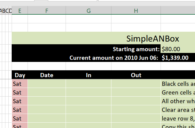
This is a financial box, a saving account, a credit, a loan, or any other financial amount that has input and output.

During my time with technology (since 1997) I found myself needing to open a lot of these boxes, to track accounts, or loans, or virtual business partnerships between multiple partnerrs. And this is the core to it.

Expenses calendar, FaCal

December 7, 2018 ANmar

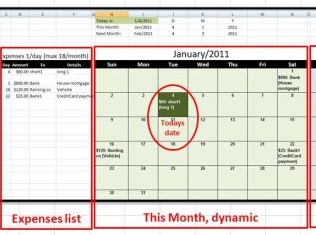
Expenses calendar, to show when in a month you need to pay what bill An easy formula-only smart sheet to allow you get hold on your bills Refreshes every time you open, to show current month and shows bills Download FaCal Excel Online

Basic Math, Conditional Formatting, DATE, Date and Time, MONTH, NETWORKDAYS, Non-functions, Standard functions, TODAY, WEEKDAY, YEAR

Custom fiscal year calendar (CFlex)

December 5, 2018 ANmar

Fully customized Yearly Calendar to show certain dates with certain format using conditional formatting, like mark 8th business day each month with certain color, 1st workday after 15th of each month, etc.
See the sheet “Data” for details and table of specific dates and rules. Contact me for more detail

Basic Math, Conditional Formatting, Data Validation, DATE, Date and Time, MONTH, Non-functions, Standard functions, TODAY, WEEKDAY, YEAR

Highlight dates dynamically

March 14, 2018 ANmar

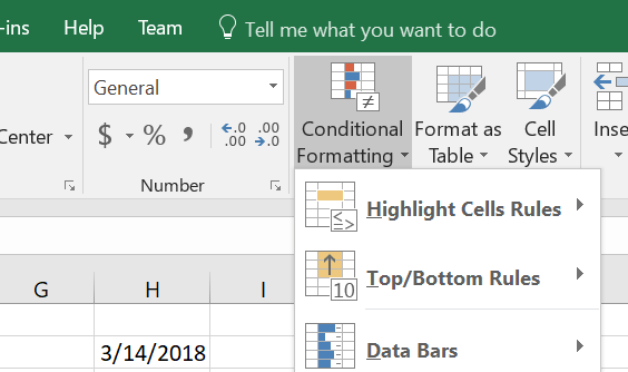
Conditional formatting is another powerful feature in Excel, especially when you combine it with functions

A simple function as in below if you set it up inside Conditional formatting, can do magic

AND, Conditional Formatting, Non-functions, Standard functions, TODAY

Week number to Month number

May 11, 2015 ANmar No Comments

Now we need to convert week number to month number

This is exactly the same as week number to date (reverse weeknum)

So, when the week number is in A5, then formula below will get you the month number

DATE, Date and Time, Formulas - combined functions, IF, Logical, MONTH, TODAY, WEEKDAY, YEAR

Week number to Sunday date – Weeknum reverse

June 17, 2014 ANmar No Comments

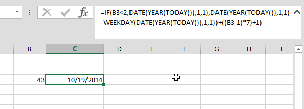
This was a request from one of my work managers
She wanted to convert a week number she got in a column into thier dates

Excel already have the WEEKNUM that converts a date into its week number, but the reverse is what needed here

So after my mouth was drooling while she was asking her question, I started a head, and below is the result formula

You just need to place the week number in cell B3, then paste this formula anywhere:

DATE, Date and Time, Formulas - combined functions, Standard functions, TODAY, WEEKDAY, WEEKNUM, YEAR