I have been asked for a while now to just put a simple VLookup function, here it is, I know this might be stupid to post it here, but we need to fill requests from all types of visitors.
Vlookup is the most famous function in Excel, some people actually refer to Excel as VLookup.
Even though I do not like that fact, especially when we have other powerful functions like INDEX, OFFSET, INDIRECT and others.
So, what is VLOOKUP?
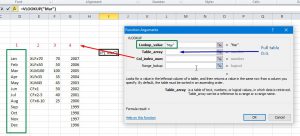
VLookup is going to search for an item in the left column of your table (or selection), as in the screenshot below, then bring me back the value in the same row where it find that item from another column.
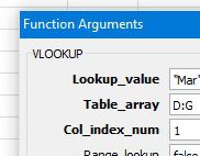
The Green box (Lookup_Value) is what the function will search for, and the vertical green box is where, this is because we selected the range (Table_Array) in Blue as the area of D:G, so VLookup will search in D, this is the V part in VLOOKUP, we should also expect to see HLookup.
Means if item is not found in column D, VLookup will return as #N/A error
The Red number (COl_Index_Num) is the number of column we need to have result from, again, because we selected D:G, if we types 1 in Col_Index_Num, we will get what is in column D that matches the same row where we found “Mar”.
In this case “Mar”
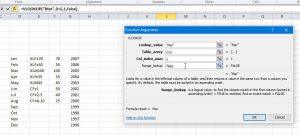
While the “Range_Lookup” is something related to the type of search, we just did “False” to make sure it searches for the exact match. to read more about “Range_Lookup”, please check the ‘Help’ section in Excel
The idea is to get result from column other than 1, this is why we are doing the search right?
So our function will be
Sample:
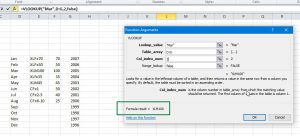
=VLOOKUP("Mar", D:G, 4, False)
And the result is as we expected.
Other ways to do Vlookup is using INDEX + MATCH or OFFSET + MATCH
