Skip to content

Excel Functions

Excel f(x)s = Excel Functions

  • Workdays – Across months DATE
  • When Excel tells you to go get some life Excel User tips
  • Excel keeps converting all cells to “Date” (or Time) Excel User tips
  • Middle name + 1st name Basic Math
  • CountIf limitation COUNTIF
  • GoLast to jump to last cell in a column CELL
  • The Excel “&” bug Excel User tips
  • Count how many times letter found Formulas - combined functions

Searching table in 2 dimensions.

Posted on July 26, 2022 By ANmar

Using VLOOKUP + MATCH (HLOOKUP + MATCH, OFFSET + 2 MATCHes or INDEX + 2 MATCHes) to search a table in both axis.

This post has been sitting for a while in my archive, waiting for me to get some time to polish and post.

Back in 1997, one of the tricks I learned and was the reason for me to start loving Microsoft Excel, is this …

Combining two (or more) functions to search a table in two dimensions.

We can use…

VLOOKUP + MATCH

Since VLOOKUP can search vertically (the V in VLOOKUP) we just need to use another function to search horizontally.

MATCH fits perfect because it returns the number of cell returned, which exactly what VLOOKUP needs
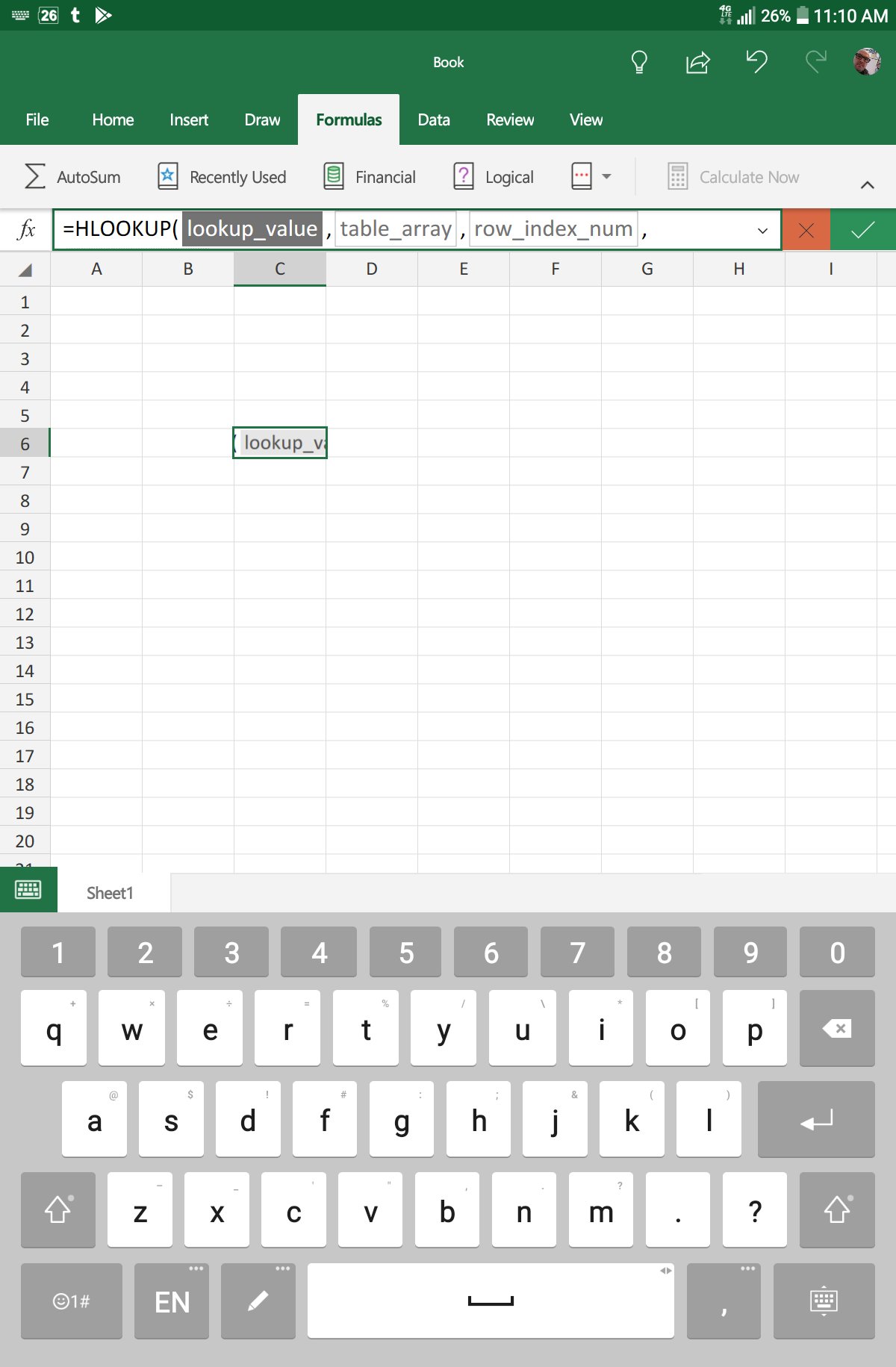
HLOOKUP + MATCH

In similar fashion, HLOOKUP will search horizontally (H in HLOOKUP), so we need a function to do the search in vertical. Yes, it is MATCH again, perfect match
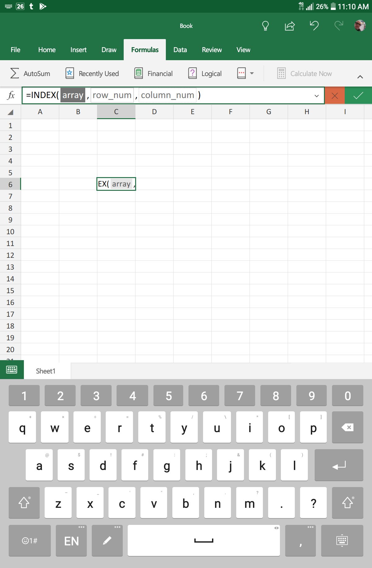
INDEX + 2 MATCHes

INDEX function does not do any search, it is basically calling the X and Y for a table, that is why we need 2 MATCHes, one vertical, and the other horizontal.

OFFSET + 2 MATCHes

OFFSET, is one of the most powerful formulas in Excel, I used it a lot (along with INDIRECT, ADDRESS, etc) to do bunch of things, here we will see how it helps us extracting from table, with the help of 2 MATCHes

We will use same table and same reference cells to show the similarities (and differences) among those 4 ways to do the search.

So, if we have our table in Sheet1, in cells B2:H22, full reference will be Sheet1!$B$2:$H$22

Then we put the ID we want to search for in vertical in Sheet2 cell B3

The column name we want to search for in Sheet2 C2

Then in C3 will be one of those formulas:

=Vlookup($B3, Sheet1!$B$2:$H$22, Match(C$2, Sheet1!$B$2:$H$2, 0), False)

=Hlookup(C$2, Sheet1!$B$2:$H$22, Match($B3, Sheet1!$B$2:$B$22, 0), False)

=Index(Sheet1!$B$2:$H$22, Match($B3, Sheet1!$B$2:$B$22, 0) +1, Match(C$2, Sheet1!$B$2:$H$2, 0) +1)

=Offset( Sheet1!$B$2, Match($B3, Sheet1!$B$2:$B$22, 0) -1, Match(C$2, Sheet1!$B$22:$H$2, 0) - 1, 1, 1)

Now that we see the 4 combination, we can easily find differences (and similarities) among them.

To describe those in English, the search funcions are VLOOKUO, HLOOKUP and MATCH.

While INDEX and OFFSET do not do any search, that is why we needed 2 MATCHes with each, while we inly needed one MATCH with VLOOKUP or HLOOKUP.

Formulas - combined functions, HLOOKUP, INDEX, Lookup and References, MATCH, Standard functions, VLOOKUP Tags:HLOOKUP, INDEX, MATCH, Search, VLOOKUP

Post navigation

Previous Post: Always get 1st name (or last)
Next Post: Comments versus Notes

Related Posts

  • Calculate hours between two cells ABS
  • Looplist – Repeating months using formulas Basic Math
  • Walking Columns ActiveX controls
  • CHOOSE – tree of decisions CHOOSE
  • Schedule column Basic Math
  • Excel @ before function names in formulas Excel User tips

Recent Posts

  • Stale values (Scratched functions)
  • Middle name + 1st name
  • LastSunday, LastSaturday
  • Paste Special Percentage
  • Jan8 date format

Archives

Categories

  • Array formula (1)
  • Formulas – combined functions (58)
  • Google Sheets (2)
  • Non-functions (36)
    • ActiveX controls (2)
    • Conditional Formatting (7)
    • Data Validation (7)
    • Excel User tips (19)
    • Format Cells (6)
    • Graphics (4)
    • Names (3)
  • Standard functions (82)
    • Basic Math (18)
    • Date and Time (16)
      • DATE (9)
      • Hour (1)
      • MONTH (7)
      • NETWORKDAYS (2)
      • TODAY (7)
      • WEEKDAY (8)
      • WEEKNUM (1)
      • YEAR (8)
    • Engineering (1)
      • CONVERT (1)
    • Information (6)
      • CELL (4)
      • ISERROR (1)
      • N (1)
    • Logical (30)
      • AND (5)
      • IF (24)
      • IFERROR (6)
      • IFNA (1)
      • IFS (1)
      • ISERROR (1)
      • OR (2)
    • Lookup and References (36)
      • ADDRESS (4)
      • CHOOSE (3)
      • COLUMN (7)
      • FORMULATEXT (1)
      • HLOOKUP (1)
      • HYPERLINK (2)
      • INDEX (5)
      • INDIRECT (6)
      • MATCH (12)
      • OFFSET (15)
      • ROW (11)
      • VLOOKUP (5)
    • Math and Trig (24)
      • ABS (1)
      • CEILING (1)
      • COUNT (1)
      • COUNTA (4)
      • INT (9)
      • LARGE (2)
      • MAX (1)
      • Min (2)
      • SMALL (3)
      • SUM (3)
      • SUMIF (1)
      • SUMIFS (2)
      • SUMPRODUCT (1)
    • Statistical (5)
      • COUNTIF (4)
      • COUNTIFS (1)
    • Texts and Strings (24)
      • CHAR (5)
      • CONCATINATE (1)
      • FIND (1)
      • LEFT (8)
      • Len (4)
      • MID (9)
      • REPT (3)
      • RIGHT (2)
      • SEARCH (9)
      • STRING (1)
      • SUBSTITUTE (2)
      • TEXT (4)
      • TRIM (2)
      • VALUE (2)
  • Uncategorized (2)
  • User-Defined f(x)s = UDF (3)
    • HyperlinkOf (1)
  • Worksheet (16)
  • XLfxs (2)

Meta

  • Log in
  • Entries feed
  • Comments feed
  • WordPress.org
  • BMI Calculator Basic Math
  • Progress bar in pure functions CHAR
  • Fixed length ID Formulas - combined functions
  • Count how many times letter found Formulas - combined functions
  • Excel Dynamic Drop-Downs that grow with you COUNTA
  • Sorting with functions only CHOOSE
  • Cuts string of list of items Formulas - combined functions
  • WorksheetName and WorksheetsNo UDFs Lookup and References

Copyright © 2025 Excel Functions.

Powered by PressBook News Dark theme